Introduction
The AEC industries have found many uses for computation. Each of the professions to adopt computational techniques have done so because it extends their capabilities;1 yet one profession remains relatively untouched by the computational paradigm: that of the landscape architect.2
A key reason for this lag is that most computational strategies focus on issues related to architectural form and building systems rather than those of land form and landscape systems. At present, landscape architects have primarily used computation to design ‘hard’ landscape elements — such as tiling patterns — where they can adopt the techniques used to design analogous architectural geometries — such as façade panelling systems. But there is a much broader range of ‘soft’ elements to landscapes that lack developed and distributed computational design techniques. This gap presents an unfilled potential for computation to drive a deeper understanding of the landscapes that can improve our designs upon the built environment.
Here we introduce some of the challenges and opportunities unique to the intersection of landscape architectural design problems and computational design methods. We discuss how landscapes present different design challenges to buildings and use a case study to test how computational techniques can be adapted to model issues of temporality and variability specific to the contemporary landscape architectural design process. In doing so, we will illustrate some of the broader benefits and challenges found in adapting computation to the design of natural systems.
The Process Discourse
Recent discussions in landscape architecture underscore the role that natural and urban processes play in the production of designed landscapes.3 Drawing from ecological science and systems theory, this discourse highlights that landscapes are comprised of complex, dynamic, and non-linear systems that emerge from processes interacting across scales and throughout time. Such a mindset drove landscape architects to develop new strategies that emphasise the design of landscape processes rather than just landscape forms.
The goal of these new methods is to “reflect the complexity and dynamism of the systems with which they engage.”4 Yet, the representational tools of landscape architecture are poorly equipped to manage this complexity and dynamism.5 Traditional maps and sections fail to display temporal change. Diagrams convey change and interaction, but do not depict their precise effects.6 Phased plans and sections are laborious to construct and modify. As a result, there is a mismatch between the conceptual aims and the practical abilities of the landscape architect. The computation design process could better align medium and message because — like landscapes — it is characterised by dynamic change.
Case Study
Creating a planting plan, when reduced to its most basic form, is an exercise in arranging circles, whereby each disc represents the average dimensions of a particular species at maturity.
This process is not dynamic. It relies on fixed and idealised averages that abstract away many of the characteristics that define landscapes as a medium and plants as a material.7 Once a building is built, the extent to which its basic form can change8 is usually limited to particular points in time where intensive modifications such as fit-outs, renovations, and extensions are designed and constructed. In contrast, a landscape changes constantly. Plants will take years, if not decades, to reach their mature states as depicted in a planting plan. The dimensions of each plant will not match the estimated averages as minute variations in highly local conditions constrain or propel their growth. Unlike a floor plan, a ‘constructed’ planting plan will never perfectly mirror the representation used to design it.
Given this inherent variability in the designed outcomes of landscapes, we should develop techniques that enable the design process to better prefigure the full range of possibilities. To demonstrate this approach, we developed an extensible Grasshopper® definition9 10 for dynamically simulating the growth and distribution of plants using parametric techniques.
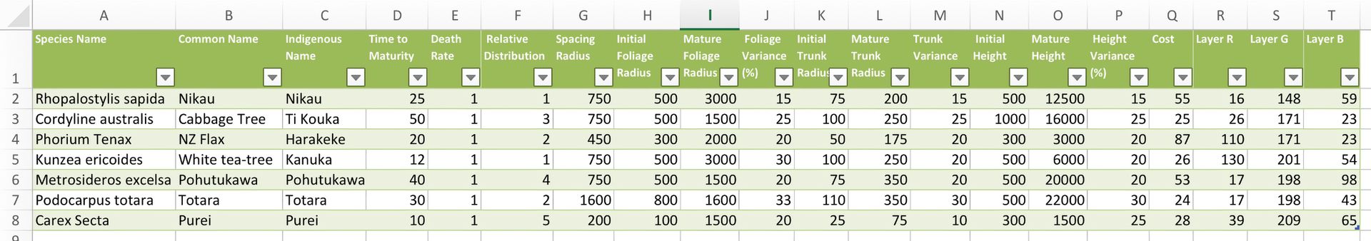
Figure .
Figure . Plants distributed within a region using circle-packing, grid divisions, and point referencing.
The first portion of this definition loads data from a comma separated value file containing a table of information (Figure 1). Each row contains attributes specific to a particular plant species such as its average growth rate, growth variance, root radius, crown radius, saturation tolerance. This information is then used to distribute plants across a surface by dividing the surface into particular grids of shapes, or through a circle packing operation (Figure 2). With either method, user-specified data such as the minimum spacing distances and relative proportions of each species are considered when distributing the plants. Alternately, groups of points in the Rhinoceros model can be referenced to precisely control placement.
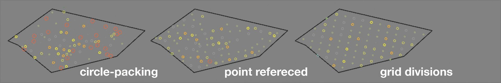
Figure .
Figure . Plants distributed within a region using various methods.
Once the surface is populated with plants, their growth can be simulated using a numeric slider that represents the passage of time after the plants are planted. The script governing this operation establishes each plant as an instance of a particular species, meaning it contains all of its species-specific attributes as well as a randomly generated number that determines how much each particular plant will differ from its species-specific averages. As a result, the dimensions of each plant of a particular species will vary in a consistent and constrained manner as the time value changes. Recalculating the definition regenerates the random seed, so that a plant that may have grown to 110% of its average height might only grow to 95% of it in a future iteration. At each specified point in time, the growth of each plant is represented using circles that depict the crown and root ball (Figure 3).
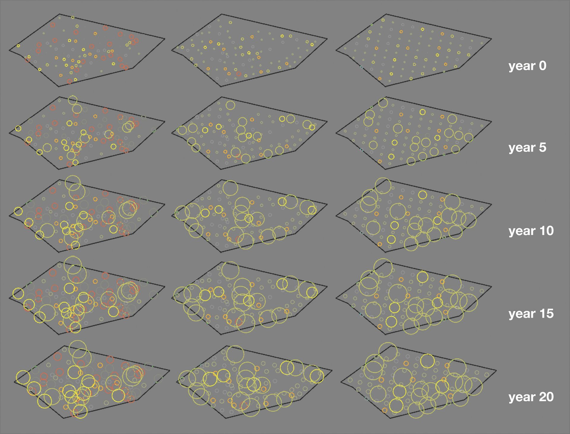
Figure .
Figure . Simulated growth of each plant instance and species at specific intervals.
Beyond simulating the growth rate of plants, the extensibility of the definition enables planting plans to be optimised according to performance criteria. As an example, the table that contains information about each species can be extended to include a tolerance value for factors such as soil saturation or terrain slope. Given a 3D model of a river and its banks, each spatial point on the site can be evaluated to determine saturation and slope values,11 which can then be cross-referenced against each species’ preferences so that the distribution algorithm places each plant in an optimal location. Similarly, the effects of the plants on their terrain could be modeled using a similar process, whereby each species could have a ‘stabilisation factor’ or ‘remediation factor’ that accrues over time and is cross-referenced to its spatial location.
Evaluation
While the methods of representation employed in this definition are relatively simple compared to those developed in computational biology, or in specialised rendering assets and setups, the ability to interactively explore how time and variability affects plants affords designers the opportunity to more rigorously test the effects of planted form in the crucial early stages of the design process. Assumptions about the eventual form and arrangement of planted areas may have been previously imagined intuitively, but by explicitly representing these assumptions they can be better tested and understood in context.
That said, the representation of organic forms within 3D-modeling environments remains a challenge. Such models need to be complex if they are to be realistic, and this complexity can seriously tax processing power.12 Furthermore, given the vast varieties of plant species specified by designers across the globe, finding an accurate 3D model for a particular species is not always possible, meaning that evaluating the nuanced aspects of plant form — such as massing, transparency, and texture — within the 3D-modeling environment typically used for architectural design remains difficult. The use of angled 2D-textures or L-Systems could provide an acceptable substitute, but relying on a designer’s intuitions and experience to judge aesthetic effects may be the most practical solution at present.
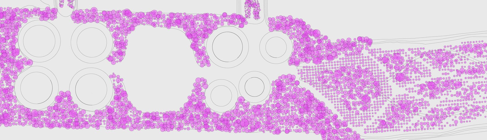
Similarly, the definition’s placement and optimisation functionality may be excessive within small-scale projects where more traditional methods of drawing (digital or otherwise) are faster than creating parametric models. However, particularly in large-scale planting projects — such as designs for ecological restoration or remediation — designers may have to distribute thousands of plants across a site (Figure 4). The use of automation can significantly accelerate the design process by front-loading key design decisions about composition and performance, while also significantly reducing the effort required to represent the resulting decisions.
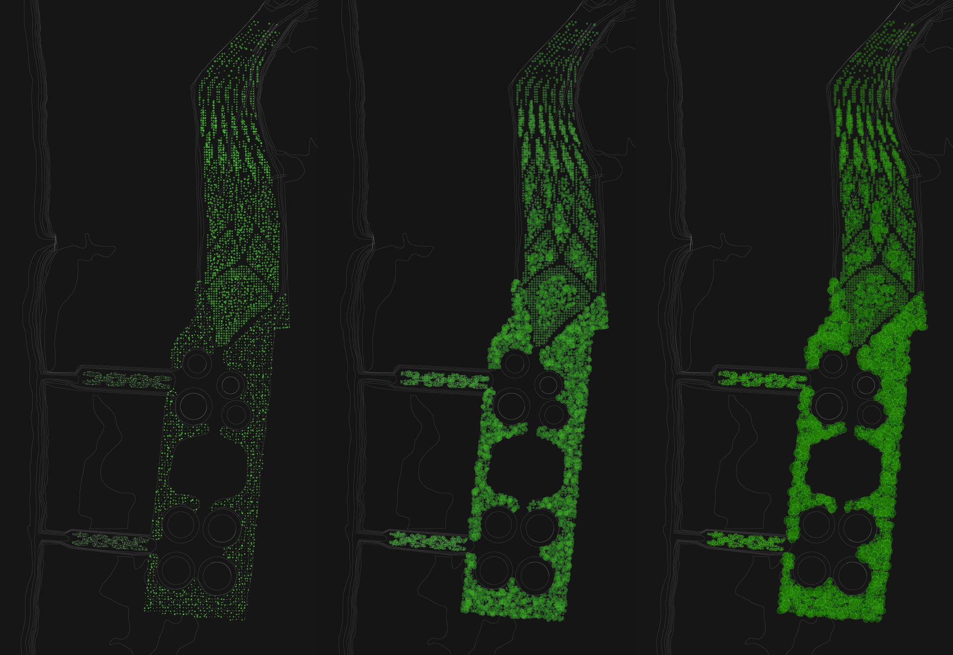
Figure .
Figure . Simulated growth, in five-year intervals, of a number of planting plan types deployed across a large site.
The results that the definition produces should be emphasised as a range of possibilities rather than a singular outcome that attempts to predict an exact result. This model doesn’t account for the fact that each plant will be heavily influenced by minute changes in its local conditions, among the many other factors that affect its growth. As such, each individually simulated plant is unlikely to grow as it is represented. However, the value of the simulation is in the aggregate display, where running several iterations gives a broad indication of the possible variations that a group of plants might collectively display. A more advanced simulation could account for the highly localised variations that more directly affect how each plant grows, although large amounts of research and interdisciplinary collaboration would be needed to create and validate such rules across a range of specific species and conditions.
Discussion
The above case-study demonstrates that the design methods of landscape architects can be achieved with speed and precision when enacted using computational methods. Computational design has helped architects tame some of the complexity involved in designing buildings, and it seems natural that it could be extended to tackle the complexities involved in designing landscapes. This approach is particularly valuable during the early stages of the design process where there is less need to represent a design with fidelity, and a larger upside to being able to run through a large set of design options rapidly.
Yet, the complexities of landscapes are different to the complexities of a building. Landscape surfaces differ from architectural surfaces in many ways, and these differences are a challenge to depict and evaluate within 3D-modelling environments. Whereas a brick can be modeled as a enclosed box with relatively uniform material properties, a patch of ground has more nuanced and less inert attributes. Properties such as saturation, pH, composition, and compaction all exists as spatial gradients that are difficult to represent with traditional forms of 3D modeling software that rely on bounded surfaces and volumes.13 In addition, the nature of landscape processes means that their complexity spans both temporal and physical scales, and that this complexity is driven by highly interrelated self-organising systems.14 For example, modeling erosion requires linking hydrological and geomorphological phenomena; it is an exercise in comparing and connecting the multitude of factors that determine soil stability against the multitude of factors that determine how water flows over landform.15 The complexity of such a simulation could quickly approach that of other notoriously difficult design problems, such of measuring the effects of architectural form on wind flows.16
But many landscape systems could be much more easily, or could be modeled in a simplified manner that nevertheless reveals important behaviours to the designer. Looking just at hydrological design tasks, the flow and absorption of groundwater, or the effects of flooding and tides, are phenomena with established models within engineering. Speaking broadly, models of landscape systems typically confined to the employ of specialists, trapped in GIS software, and delayed until the latter stages of the design process. As architects now use computational techniques that employ advanced models from physics and material science to create and validate form against function early in the design process, so too should landscape architects begin to adopt and adapt models that can test the temporality and variability present within the landscapes they design.
Conclusion
This is a small case study into a much larger project to develop computational design techniques that can empower landscape architects. But this broader task has significant challenges: landscapes and buildings have different formal conditions, and landscape systems are unlike those of architecture systems. The difficulties in representing landscapes in common 3D-modeling software and the lack of established and validated landscape-specific techniques means much work is needed if computation is to play a significant role in landscape architecture. That said, the pay-off for doing so could be large. Landscape architecture has long emphasised the need to account for temporality and variability within the design process, but often struggles with the complexities entailed in representing and evaluating these aspects. Computation can offer a solution.
- Mark Burry and Andrew Maher, “The Parametric Bridge,” in ACADIA 22, 2003, 39–47.↩
- Charles Waldheim, “Landscape as Digital Media,” June 21, 2013, http://www.multimedia.ethz.ch/conferences/2013/ila/06_friday.↩
- Julian Raxworthy, “Novelty in the Entropic Landscape” (The University of Queensland, 2013).↩
- J Margaretts, Rod Barnett, and N Popov, “Landscape Systems Modelling,” in Proceedings of the 13th Annual Australia and New Zealand Systems Conference, ed. J Shepherd and K Fielder, 2007, 1–10.↩
- Sue-Anne Ware, “Representation, Generation and Emancipation in Virtual Landscapes,” Landscape Review 8, no. 1 (2003): 3–11.↩
- Peter Connolly, “What Is Design Research in Landscape Architecture?” in Technique (RMIT University Press, 2002), 20–33.↩
- Julian Raxworthy, “Novelty in the Entropic Landscape” (The University of Queensland, 2013).↩
- With the notable exception of kinetic architecture; a field whose design process has much in common with landscape architecture.↩
- Most of the logic of the definition is contained within Python code embedded into GhPyhon components. These components, and others, form part of an unreleased plugin — Badger — that focuses on implementing landscape architectural design techniques and tactics.↩
- Many researches within computer graphics and computational biology have created similar, much more advanced models, as have architectural researchers, such as Takenaka, Tsukasa, and Aya Okabe in “Development of the Seed Scattering System for Computational Landscape Design, International Journal of Architectural Computing 9, no. 4 (February 8, 2012): 421–436. This approach differs in that rather than developing a highly detailed model tailored to a particular site and context, it aims to create a generic, but extensible, model that can be easily adapted to a wide range of contexts and can integrate with the established and widespread workflows of Grasshopper®.↩
- The terrain slope can be determined by finding the surface normal, while soil saturation can be estimated by determining each point’s distance from the average bounds of the river.↩
- Sören Pirk et al., “Plastic Trees,” ACM Transactions on Graphics 31, no. 4 (2012): 50.↩
- J Margaretts, Rod Barnett, and N Popov, “Landscape Systems Modelling,” in Proceedings of the 13th Annual Australia and New Zealand Systems Conference, ed. J Shepherd and K Fielder, 2007, 1–10.↩
- J Margaretts, Rod Barnett, and N Popov, “Landscape Systems Modelling,” in Proceedings of the 13th Annual Australia and New Zealand Systems Conference, ed. J Shepherd and K Fielder, 2007, 1–10.↩
- Julian Raxworthy, “Novelty in the Entropic Landscape” (The University of Queensland, 2013).↩
- ‘Hard’ in the sense that valid results requires expertise to setup the initial parameters of the simulation, and that high-fidelity simulations can consume large amounts of computational resources.↩